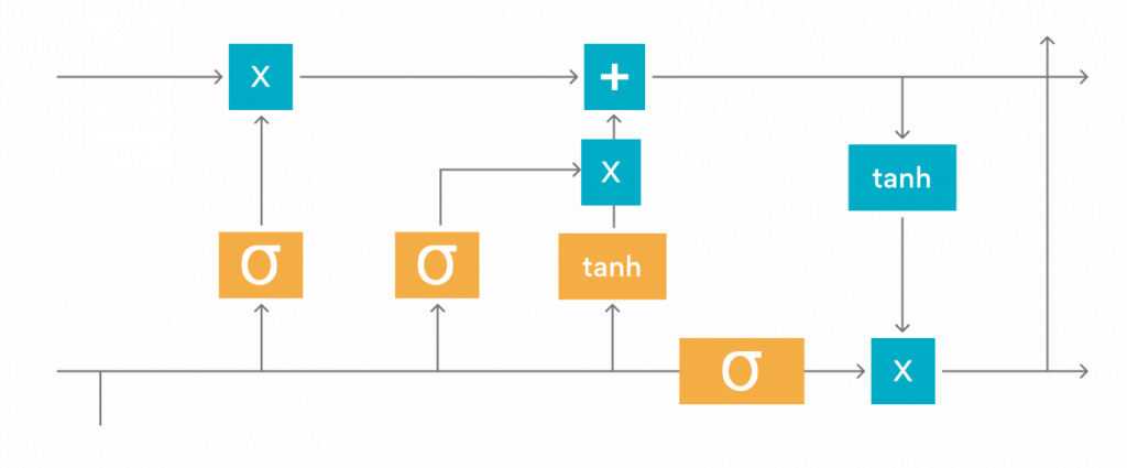
Long short-term memory (LSTM) is an artificial recurrent neural network (RNN) architecture used widely in deep learning. These networks classify, process, and make predictions based on time-series datasets that could contain hidden information between important events.
Unlike the standard feed-forward neural networks, LSTMs have feedback connections. Along with processing single data points, like images, LSTM can also process entire sequences of data, like – speech and video. They can also be applied to tasks such as connected, unsegmented handwriting recognition
While studying LSTM, I came across long-winded codes that increased the complexity of model training. Through this post, I intend to share a shorter, simpler yet effective implementation of LSTMs for training a predictive model with historic current-hour sales data.
Before starting the development of the sales prediction model, let me take you through the high-level steps to train any kind of a model,
- Identifying the problem and deciding if resolving it through Machine Learning is feasible.
- Gathering good amount of data and data exploration.
- Cleaning the data and performing feature engineering, if required.
- Designing the model by defining its architecture, what features will it accept, and the functions and filters needed to train the model.
- Evaluating trained model and changing the parameters to improve the accuracy of model.
In the context of the problem I have chosen, this is how the result of each step looks like –
- Finding the problem: The problem statement is — To predict the next hour sales of a store based on the current hour sales data and to implement the model using LSTM.
- Gathering data and exploration: I got basic liquor sales data from here. I made some modifications in data for direct use. To reduce the complexity of the dataset for the blog, I reduced the huge raw data of multiple stores to just one store’s data. To access this data, please refer to my git repo. Read the ‘LiquorSales.csv’ file using pandas library.
df = pd.read_csv('LiquorSales.csv')
df.head()

- Cleaning the data and feature engineering : The code below was used to customize the data. As the data was already customized, so cleaning of data wasn’t required. From Table 1, we can easily determine that hour, date, and month are categorical features, whereas quantity column is a continuous feature. So, I performed feature engineering over these two feature types using one-hot encoding and normalization, respectively.
# Max and min values help in feature normalization.
max_quantity = df['quantity'].max()
min_quantity = df['quantity'].min()
# Perform One-hot encoding on categorical columns and normalize continuous column.
df = pd.get_dummies(data=df, columns = ['hour', 'date','month'])
# Normalize the continuous column.
df['quantity'] = (df['quantity']-min_quantity)/(max_quantity-min_quantity)
df_quan = pd.DataFrame(columns=['quantity'])
df_quan.quantity = df.quantity
df.head()

Before starting to design the model, I distributed the data into training, validation and test with the following code.
df_x = df.to_numpy()
df_y = df_quan.to_numpy()
# separate into train validation and testing data.
x_train, x_test, y_train, y_test = train_test_split(df_x, df_y, test_size=0.2, shuffle= False)
x_train, x_val, y_train, y_val = train_test_split(x_train, y_train, test_size=0.25, shuffle= False)
x_train = x_train[:-1]
x_val = x_val[:-1]
x_test = x_test[:-1]
y_train = y_train[1:]
y_val = y_val[1:]
y_test = y_test[1:]
print(x_train.shape, x_val.shape, x_test.shape,
      y_train.shape, y_val.shape, y_test.shape)
To train the LSTM model, I converted the data into a 3D array with these attributes — (samples, timesteps, features).
train_x = x_train.reshape((x_train.shape[0], 1, x_train.shape[1]))
test_x = x_test.reshape((x_test.shape[0], 1, x_test.shape[1]))
val_x = x_val.reshape((x_val.shape[0], 1, x_val.shape[1]))
print(train_x.shape, val_x.shape, test_x.shape,
      y_train.shape, y_val.shape, y_test.shape)
- Designing the model: I designed a basic LSTM model to train effectively on my prepared data. These were the parameters that I used to train the model,
Epoch : It is the number of times the learning algorithm will go through the entire training dataset. I took 1500 as the epoch value.
Batch Size : It is the number of samples to go through before updating the internal model parameters. I took 256 as the batch size.
Learning Rate : It helps to control by how much to change the model with respect to the estimated error after each time the model weights are updated. I took a small learning rate of 0.003.
Decay : The amount by which the learning rate changes over training epochs is termed as the learning rate decay. Since my data was simple and clean, I took the decay value as 0.
Neurons : Here neurons are the number of hidden units inside the LSTM cell. Also it could be considered as the positive integer with the dimensionality of the output space. I could have taken these neurons as 1, but since the input was of 68 features, I considered a higher number of 17 for neurons.
Output Neurons : Here output neurons are considered as the number of output units. In this case, the model output is the prediction of the quantity of liquor sold in the next hour. This is done with the help of DENSE function in keras to link LSTM output units with dense layer at the end. Therefore, I set it as 1.
Dropout : It is a technique where randomly selected neurons are ignored during training. It is used when a model overfits. I took the dropout as 0 since mine was a simple model.
I chose Adam optimizer for our model. It requires very little memory and is computationally efficient. It is recommended to use Adam Optimizer for regression models.
# Setting parameters for model and begin training
epoch = 1500
batch = 256
decay = 0
learning_rate = 0.003
neurons = 17
dropout = 0
output_neurons = 1
version = 0
# Name of model file to be saved
file_path = "./Liquor_ckpt" \
            + "_V" + str(version) \
            + "_L1_" + str(neurons) \
            + "_Dro1_" + str(dropout) \
            + "_De1_" + str(output_neurons) \
            + "a.hdf5"
# Model architecture
model = Sequential()
model.add(LSTM(neurons, input_shape=(1, train_x.shape[2]), return_sequences=False, name='L1'))
# We could add dropout in layers if model overfits.
# model.add(Dropout(dropout,  name='Dro1'))
model.add(Dense(output_neurons, name='De1'))
# We could add activation function for better learning of model.
# model.add(Activation('relu'))
adam = optimizers.Adam(lr=learning_rate, decay=decay)
model.compile(loss='mean_squared_error', optimizer=adam)
# Using checkpoint to save only 1 model that fits best on validation data.
checkpoint = ModelCheckpoint(file_path, monitor='val_loss', verbose=1,
 save_best_only=True, mode='auto', period=1)
history = model.fit(train_x, y_train, batch_size=batch, epochs=epoch,
 verbose=2, validation_data=(val_x, y_val), callbacks=[checkpoint])
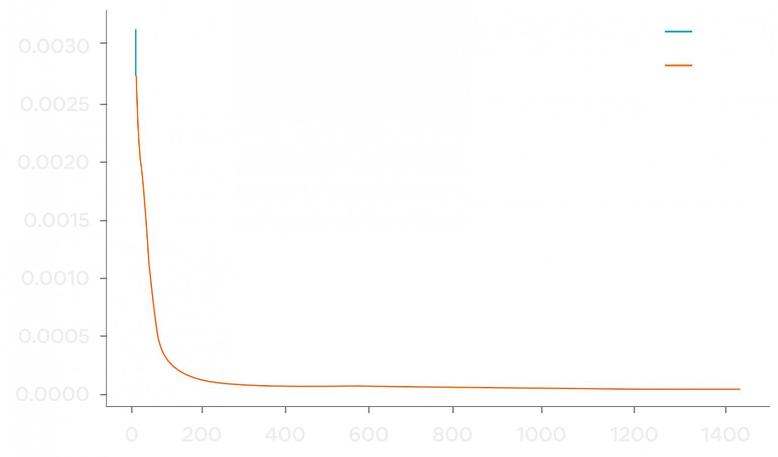
- Evaluate trained model: I evaluated the convergence of the model by plotting the epochs vs loss graph.
# Plot epoch loss graph
plt.plot(history.history['loss'], label='train')
plt.plot(history.history['val_loss'], label='test'
plt.legend()
plt.figure(figsize=(10,8),dpi=80)
plt.show()

Then I predicted the quantity which could be sold in the next hour. Using the test data, I also plotted a graph of actual sold VS sales prediction.
# Load Model
# file_path = "Liquor_ckpt_V0_L1_17_Dro1_0_De1_1a.hdf5"
model1 = load_model(file_path)
predicted = model1.predict(test_x)
# Reconstruct original values
test_y1 = (y_test * (max_quantity-min_quantity)) + min_quantity
pred_Model_1 = (predicted * (max_quantity-min_quantity))
               + min_quantity
plt.figure(figsize=(20,5),dpi=80)
plt.plot(test_y1[:200], 'r',label='Actual')
plt.plot(pred_Model_1[:200], 'g', label='Predicted')
plt.legend()
plt.show()

Then, I calculated the R2 score to check the accuracy of the model.
score = r2_score(test_y1, pred_Model_1)
print('r2 score for model 1 : ',score)
The model achieved a really good R2 score of 0.998 that meant the model was trained well with the selected simple and clean dataset.
You can access the source code, data set, and trained model you can get it here.
If you plan to work on complex data, you could do any of the following tweaks to the parameters to achieve a well-trained model,
- Changing epoch for training until the model reaches convergence.
- Changing batch size depending on the system where training is to be executed.
- Tweaking learning rate and learning rate decay.
- Introduce dropout layer.
- Introduce activation function.
- Introduce more LSTM and Dense layers and much more.
If you like the post, drop a few claps and suggest ideas for complex LSTM implementation that you would like to see in the later posts in the comment section.


